CarND-Vehicle-Detection
View the Project on GitHub MarkBroerkens/CarND-Vehicle-Detection

The Project
The goals / steps of this project are the following:
- Perform a Histogram of Oriented Gradients (HOG) feature extraction on a labeled training set of images and train a Linear SVM classifier
- Apply a color transform and append binned color features, as well as histograms of color
- Implement a sliding-window technique and use a trained classifier to search for vehicles in images.
- Run your pipeline on a video stream and create a heat map of recurring detections frame by frame to reject outliers and follow detected vehicles.
- Estimate a bounding box for vehicles detected.
Overview of Files
My project includes the following files:
- README.md (writeup report) documentation of the results
-
L_project_video.mp4 the movie that shows the detected vehicles
- car_finder_pipeline.py the pipeline that for vehicle detection
- hotspots.py implementation of heatmap
- image_util.py utility for loading and saving of images
- lesson_functions.py some functions from the lesson
- search_and_classify.py detection of vehicles in images
- train.py code for training the classifier
- train_pickle.p saved classifier including the parmeters that have been used for training and feature extraction
- videoprocess.py processes the video
Feature Extraction and Training of Classfier
Feature extraction from the training images
The code for training the classifier is defined in function train() in file train.py. This function is invoked with a list of file names of vehicle and non-vehicle images and several parameters that configure the feature extraction algorithms.
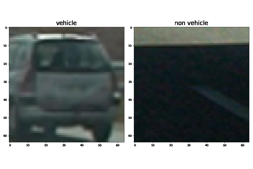
Here is an example of one of each of the vehicle and non-vehicle classes:
In order to identify if the images that show a vehicle the following feature extraction techniques are used:
- Histogram of Color
- Spatial Binning
- Histogram of oriented gradients
Histograms of Color
The combinations of parameters and its impact on the test accuracy is calculated in test test_01_train_histogram() of test_train.py
| Number of features | Color space | Numer of bins | Test Accuracy |
|---|---|---|---|
| 24 | RGB | 8 | 0.842 |
| 48 | RGB | 16 | 0.884 |
| 96 | RGB | 32 | 0.902 |
| 192 | RGB | 64 | 0.922 |
| 24 | HSV | 8 | 0.906 |
| 48 | HSV | 16 | 0.946 |
| 96 | HSV | 32 | 0.947 |
| 192 | HSV | 64 | 0.952 |
| 24 | LUV | 8 | 0.868 |
| 48 | LUV | 16 | 0.889 |
| 96 | LUV | 32 | 0.910 |
| 192 | LUV | 64 | 0.932 |
| 24 | HLS | 8 | 0.888 |
| 48 | HLS | 16 | 0.921 |
| 96 | HLS | 32 | 0.948 |
| 192 | HLS | 64 | 0.961 |
| 24 | YUV | 8 | 0.865 |
| 48 | YUV | 16 | 0.889 |
| 96 | YUV | 32 | 0.911 |
| 192 | YUV | 64 | 0.930 |
| 24 | YCrCb | 8 | 0.873 |
| 48 | YCrCb | 16 | 0.883 |
| 96 | YCrCb | 32 | 0.923 |
| 192 | YCrCb | 64 | 0.936 |
Spatial Binning
The combinations of parameters and its impact on the test accuracy is calculated in test test_02_train_spatial of test_train.py
| Number of features | Color space | Spartial Size | Test Accuracy |
|---|---|---|---|
| 192 | RGB | 8 | 0.902 |
| 768 | RGB | 16 | 0.905 |
| 3072 | RGB | 32 | 0.909 |
| 12288 | RGB | 64 | 0.905 |
| 192 | HSV | 8 | 0.873 |
| 768 | HSV | 16 | 0.899 |
| 3072 | HSV | 32 | 0.872 |
| 12288 | HSV | 64 | 0.877 |
| 192 | LUV | 8 | 0.898 |
| 768 | LUV | 16 | 0.926 |
| 3072 | LUV | 32 | 0.901 |
| 12288 | LUV | 64 | 0.904 |
| 192 | HLS | 8 | 0.871 |
| 768 | HLS | 16 | 0.895 |
| 3072 | HLS | 32 | 0.870 |
| 12288 | HLS | 64 | 0.877 |
| 192 | YUV | 8 | 0.901 |
| 768 | YUV | 16 | 0.919 |
| 3072 | YUV | 32 | 0.901 |
| 12288 | YUV | 64 | 0.896 |
| 192 | YCrCb | 8 | 0.899 |
| 768 | YCrCb | 16 | 0.924 |
| 3072 | YCrCb | 32 | 0.896 |
| 12288 | YCrCb | 64 | 0.901 |
The best results are marked in the table.
Gradient Features
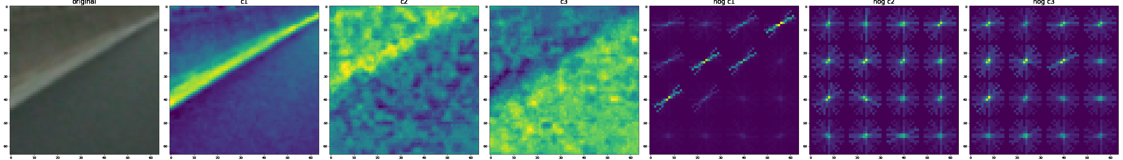
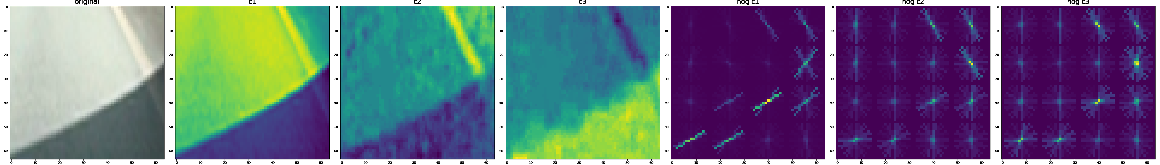
Histograms of Ordered Gradients (HOG) were calculated in order to extract features that represent the shape of the vehicle.
I explored different color spaces and different skimage.hog() parameters (orientations, pixels_per_cell, and cells_per_block).
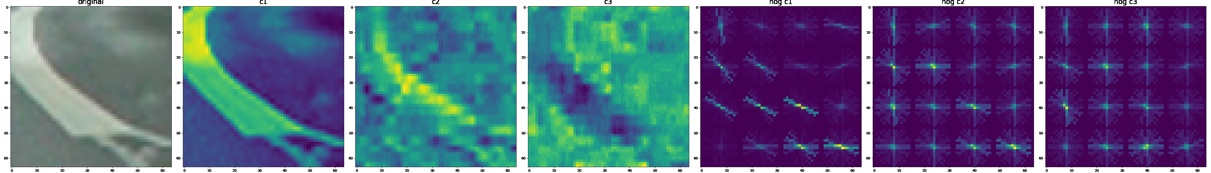
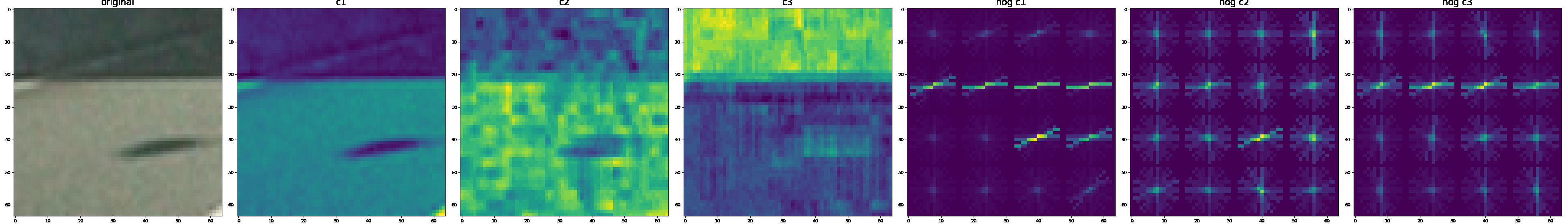
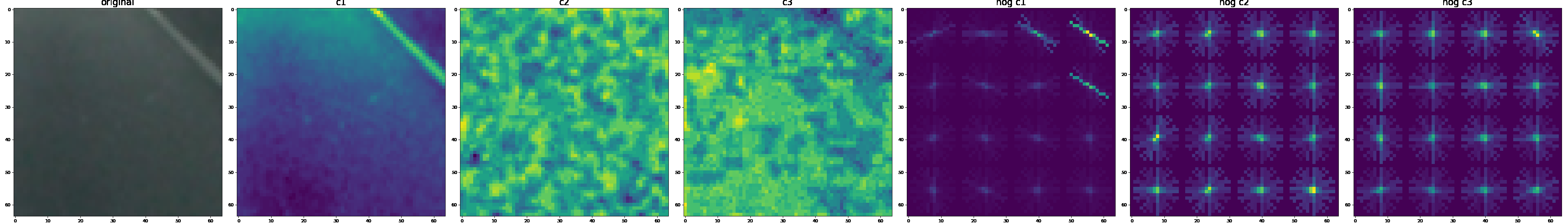
Here are example using the YUV color space and HOG parameters of orientations=13, pixels_per_cell=(16, 16) and cells_per_block=(2, 2):
Examples of vehicels
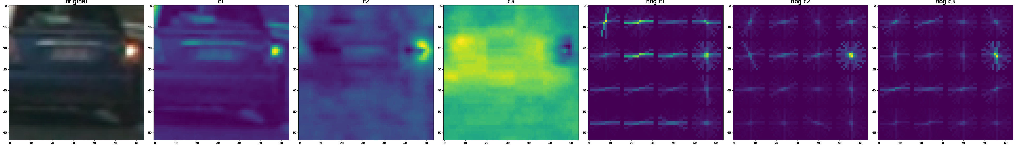
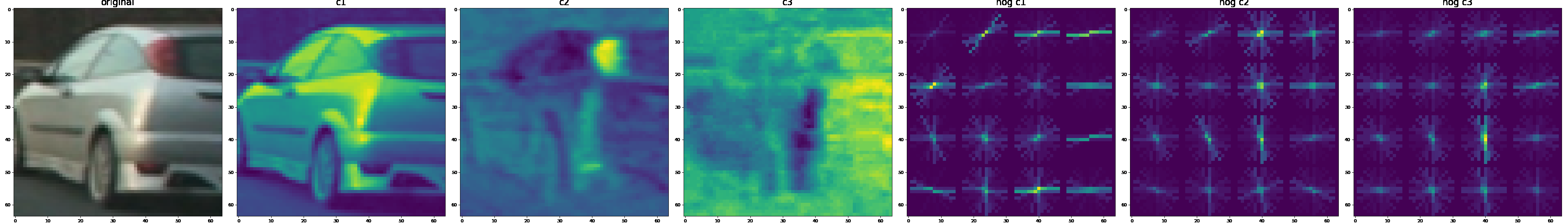
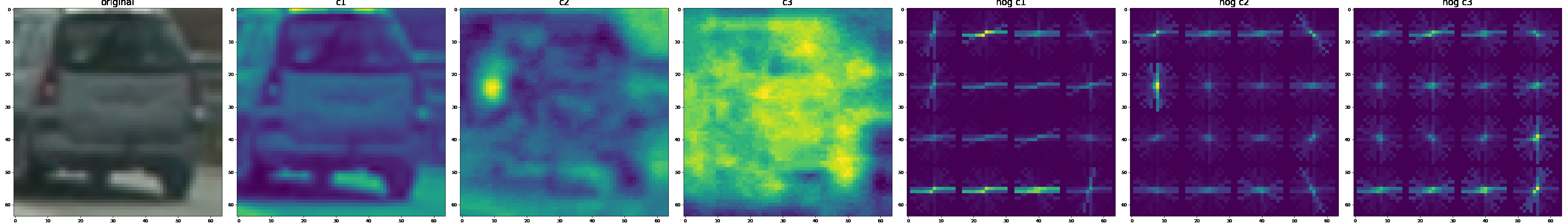
Exemples of non vehicles
A linear Support Vector Machine classifier was trained with feature vectors that were created by different skimage.hog() parameters in order to figure out which parameters work best on the given training data. The following table is calculated in test_03_train_hog() of test_train.py
| len features | color_space | orient | pix_per_cell | cell_per_block | hog_channel | accuracy |
|---|---|---|---|---|---|---|
| 2940 | HSV | 5 | 8 | 2 | ALL | 0.962 |
| 6000 | HSV | 5 | 8 | 4 | ALL | 0.965 |
| 540 | HSV | 5 | 16 | 2 | ALL | 0.971 |
| 240 | HSV | 5 | 16 | 4 | ALL | 0.969 |
| 5292 | HSV | 9 | 8 | 2 | ALL | 0.955 |
| 10800 | HSV | 9 | 8 | 4 | ALL | 0.950 |
| 972 | HSV | 9 | 16 | 2 | ALL | 0.973 |
| 432 | HSV | 9 | 16 | 4 | ALL | 0.969 |
| 7644 | HSV | 13 | 8 | 2 | ALL | 0.942 |
| 15600 | HSV | 13 | 8 | 4 | ALL | 0.945 |
| 1404 | HSV | 13 | 16 | 2 | ALL | 0.968 |
| 624 | HSV | 13 | 16 | 4 | ALL | 0.968 |
| 2940 | LUV | 5 | 8 | 2 | ALL | 0.967 |
| 6000 | LUV | 5 | 8 | 4 | ALL | 0.968 |
| 540 | LUV | 5 | 16 | 2 | ALL | 0.976 |
| 240 | LUV | 5 | 16 | 4 | ALL | 0.975 |
| 5292 | LUV | 9 | 8 | 2 | ALL | 0.965 |
| 10800 | LUV | 9 | 8 | 4 | ALL | 0.966 |
| 972 | LUV | 9 | 16 | 2 | ALL | 0.976 |
| 432 | LUV | 9 | 16 | 4 | ALL | 0.977 |
| 7644 | LUV | 13 | 8 | 2 | ALL | 0.969 |
| 15600 | LUV | 13 | 8 | 4 | ALL | 0.969 |
| 1404 | LUV | 13 | 16 | 2 | ALL | 0.983 |
| 624 | LUV | 13 | 16 | 4 | ALL | 0.976 |
| 2940 | HLS | 5 | 8 | 2 | ALL | 0.957 |
| 6000 | HLS | 5 | 8 | 4 | ALL | 0.966 |
| 540 | HLS | 5 | 16 | 2 | ALL | 0.972 |
| 240 | HLS | 5 | 16 | 4 | ALL | 0.962 |
| 5292 | HLS | 9 | 8 | 2 | ALL | 0.949 |
| 10800 | HLS | 9 | 8 | 4 | ALL | 0.952 |
| 972 | HLS | 9 | 16 | 2 | ALL | 0.972* |
| 432 | HLS | 9 | 16 | 4 | ALL | 0.968 |
| 7644 | HLS | 13 | 8 | 2 | ALL | 0.944 |
| 15600 | HLS | 13 | 8 | 4 | ALL | 0.949 |
| 1404 | HLS | 13 | 16 | 2 | ALL | 0.967 |
| 624 | HLS | 13 | 16 | 4 | ALL | 0.969 |
| 2940 | YUV | 5 | 8 | 2 | ALL | 0.965 |
| 6000 | YUV | 5 | 8 | 4 | ALL | 0.969 |
| 540 | YUV | 5 | 16 | 2 | ALL | 0.976 |
| 240 | YUV | 5 | 16 | 4 | ALL | 0.978 |
| 5292 | YUV | 9 | 8 | 2 | ALL | 0.967 |
| 10800 | YUV | 9 | 8 | 4 | ALL | 0.975 ] |
| 972 | YUV | 9 | 16 | 2 | ALL | 0.980 |
| 432 | YUV | 9 | 16 | 4 | ALL | 0.978 |
| 7644 | YUV | 13 | 8 | 2 | ALL | 0.980 |
| 15600 | YUV | 13 | 8 | 4 | ALL | 0.970 |
| 1404 | YUV | 13 | 16 | 2 | ALL | 0.981 |
| 624 | YUV | 13 | 16 | 4 | ALL | 0.973 |
| 2940 | YCrCb | 5 | 8 | 2 | ALL | 0.964 |
| 6000 | YCrCb | 5 | 8 | 4 | ALL | 0.969 |
| 540 | YCrCb | 5 | 16 | 2 | ALL | 0.976 |
| 240 | YCrCb | 5 | 16 | 4 | ALL | 0.980 |
| 5292 | YCrCb | 9 | 8 | 2 | ALL | 0.967 |
| 10800 | YCrCb | 9 | 8 | 4 | ALL | 0.967 |
| 972 | YCrCb | 9 | 16 | 2 | ALL | 0.976 |
| 432 | YCrCb | 9 | 16 | 4 | ALL | 0.976 |
| 7644 | YCrCb | 13 | 8 | 2 | ALL | 0.970 |
| 15600 | YCrCb | 13 | 8 | 4 | ALL | 0.974 |
| 1404 | YCrCb | 13 | 16 | 2 | ALL | 0.977 |
| 624 | YCrCb | 13 | 16 | 4 | ALL | 0.979 |
The best results are marked in the table.
Combination of Feature Extraction
color space YUV number of orientations=13, pix per cell 16, cells per block 2, and hog channels = “All”, spartial size of 16, 64 bins.
| len features | spatial_feat | hist_feat | hog_feat | accuracy |
|---|---|---|---|---|
| 2364 | True | True | True | 0.991 |
| 960 | True | True | False | 0.961 |
| 2172 | True | False | True | 0.986 |
| 768 | True | False | False | 0.924 |
| 1596 | False | True | True | 0.990 |
| 192 | False | True | False | 0.933 |
| 1404 | False | False | True | 0.983 |
The best results are marked in the table.
Training of the Classifier
I trained a linear SVM using the following test data that consists of 8792 vehicle images and 8968 non vehicles images
The training of the classifier is implemented in function train() of train.py:
- For each image the feature vector is calculated in method
extract_features()in that is implemented in file lesson_functions.py: sklearn.preprocessing.StandardScaler()is used to normalize the feature vectorssklearn.model_selection.train_test_split()creates shuffled training and test data and labels- the trained classifier is is saved via pickle so that it can be reused later (see test_train.py )
Sliding Window Search
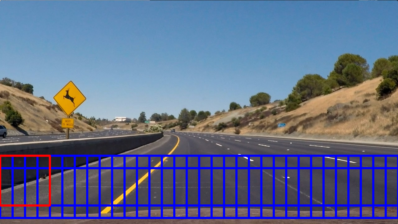
The trained classifier is applied on sliding windows of different sizes. Small sizes are applied in parts of the image where the vehicles are expected to be small. Bigger windows are used at the lower part of the image where they are expected to be big.
- ystart = 380
- ystop = 480
-
scale = 1.0
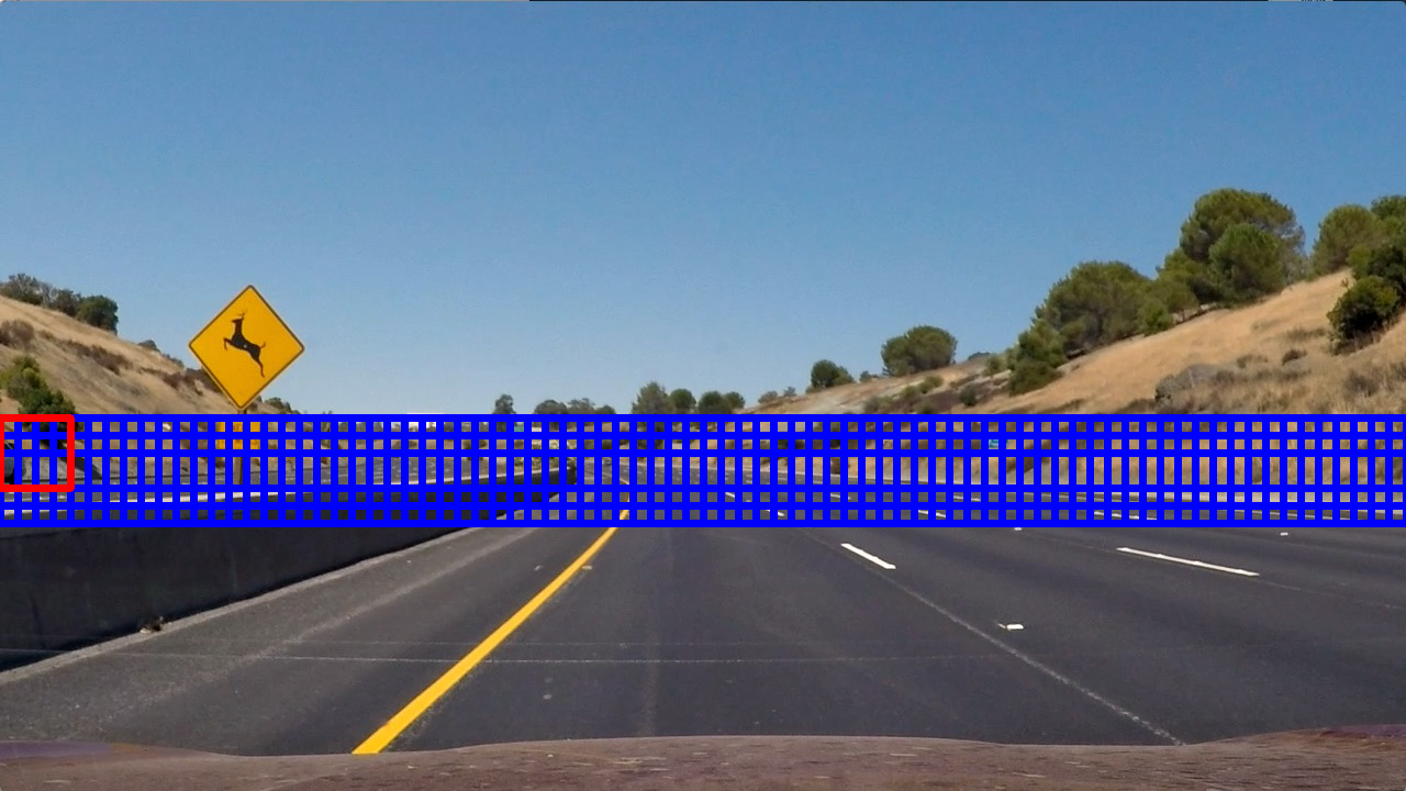
- ystart = 400
- ystop = 600
-
scale = 1.5
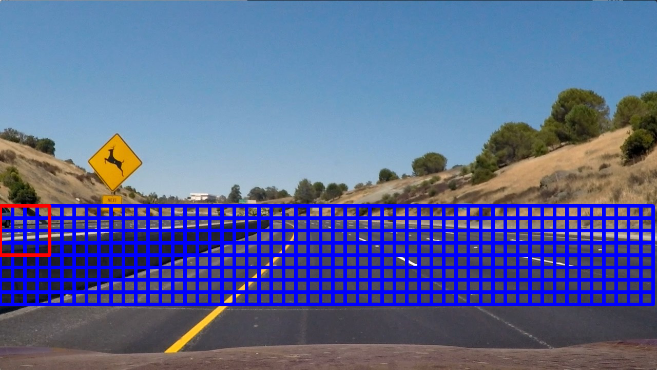
- ystart = 500
- ystop = 700
- scale = 2.5
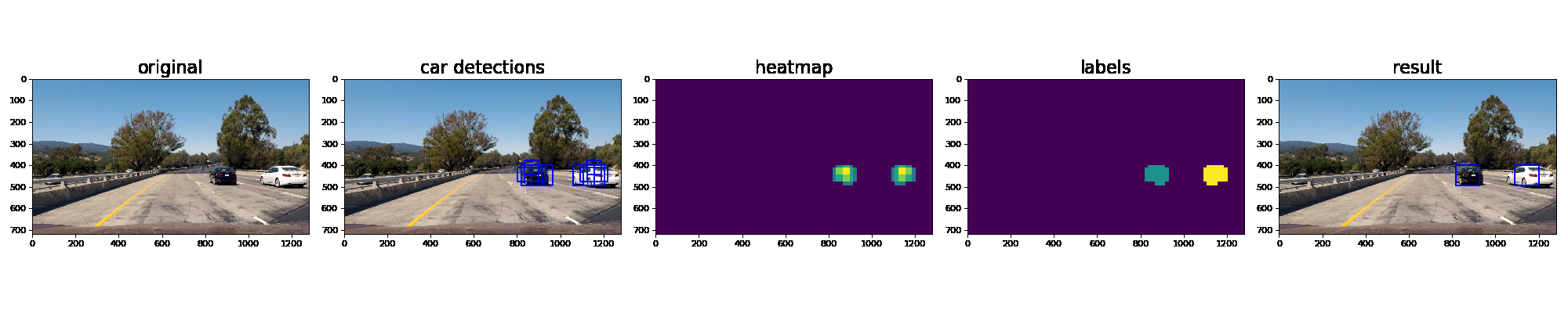
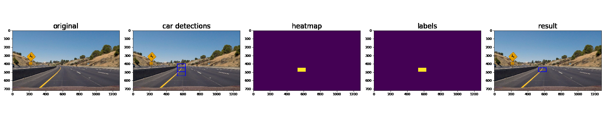
The pipeline for detection of cars is implemented in function process() in file car_finder_pipeline.py. It consists of the following steps:
- Search for vehicles using the aformentioned sliding windows approach (see the
find_cars()that is implemented in search_and_classify.py ) - If the classifier detects a car in the window, then the window is added to the set of
hotboxes. - These boxes are then combined in a heatmap that shows how many boxes overlap at each point in the image.
- I then used
scipy.ndimage.measurements.label()to identify individual blobs in the heatmap (see hotspots.py). - I then assumed each blob corresponded to a vehicle. I constructed bounding boxes to cover the area of each blob detected.
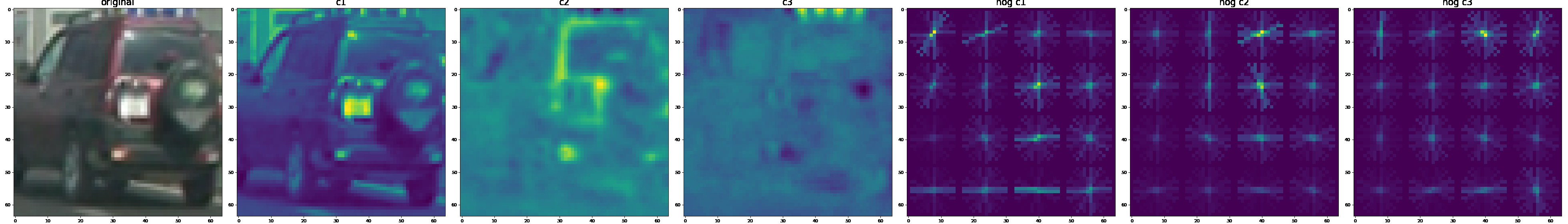
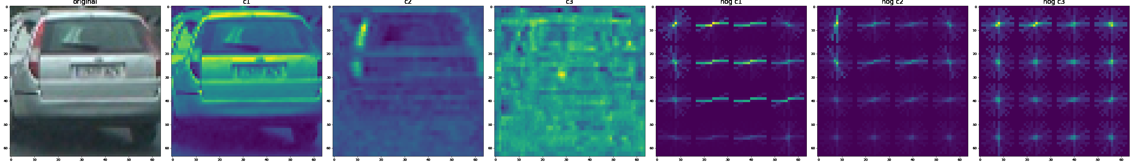
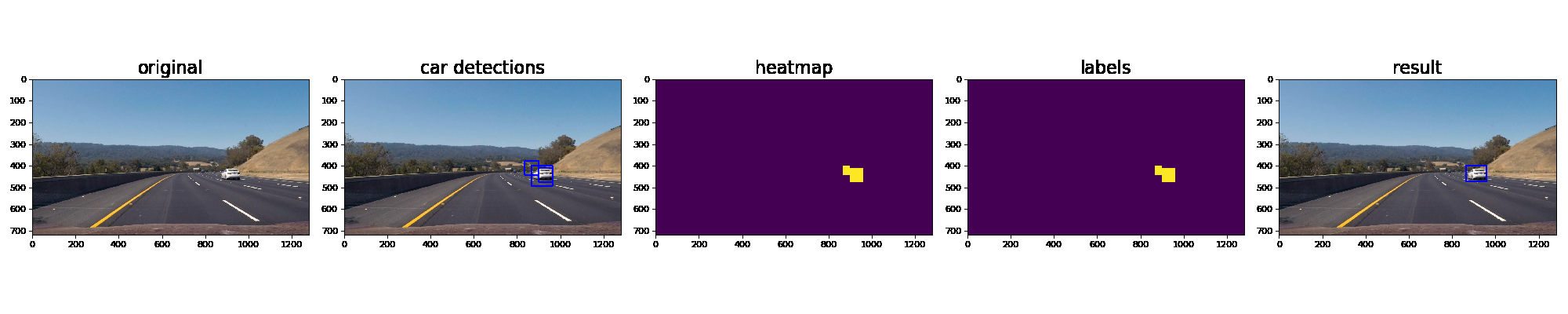
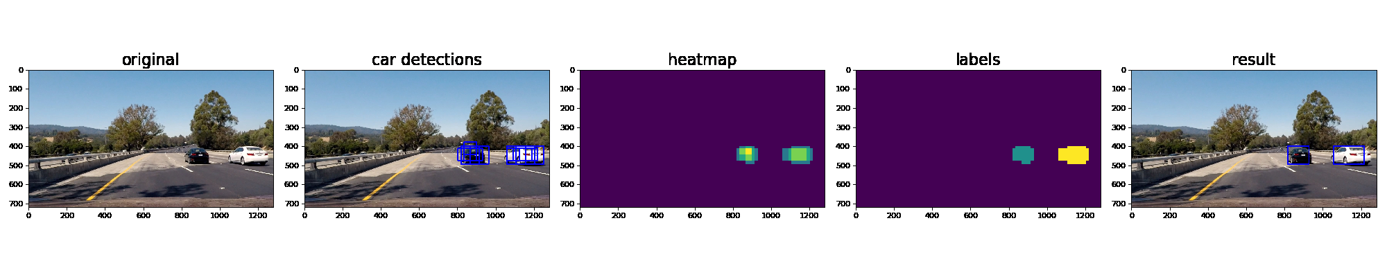
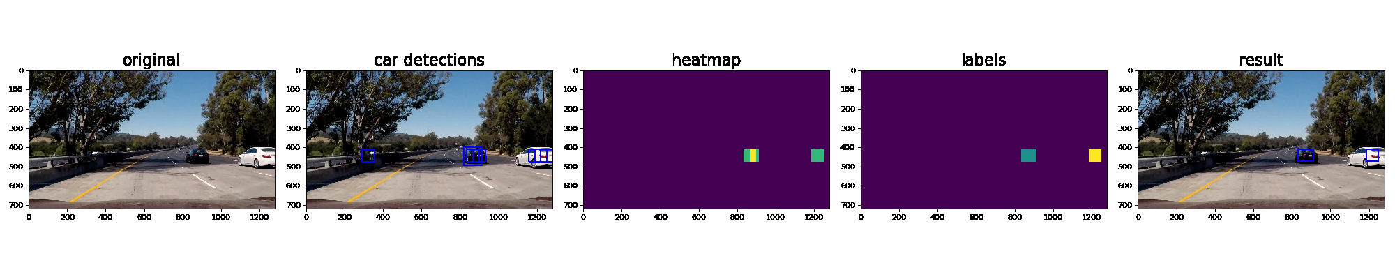
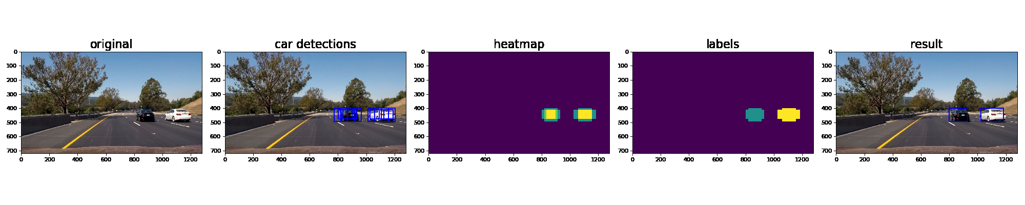
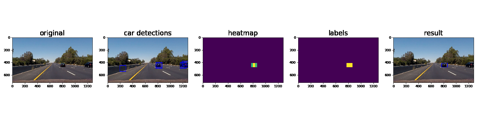
Ultimately I searched on three scales using YUV 3-channel HOG features plus spatially binned color and histograms of color in the feature vector, which provided a nice result. Here are some example images of the results and the intermediate calculations:
Video Implementation
Here’s a link to my video result
In order to reduce the false positives I included detections of vehicles in previous frames (see hotspots.py, draw_labeled_bboxes_with_history())
Here’s an example showing results and the intermediate work product of a sequence of frames in the project video.:


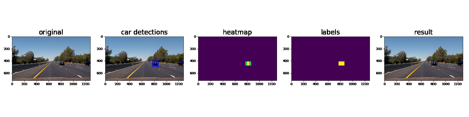


Here the resulting bounding boxes are drawn onto the last frame in the series:
Discussion
While implementing this project I frequently ran into the situation where I tried to reuse a classifier that was trained using different feaure extraction strategies and parameters. By adding the parameters into the pickle file, I was able to avoid this problem.
The results of the vehicle detections improved significantly by improving the following aspects of the code:
- improve accuracy of classifier
- eleminiation of false positives by considering the hotspots of the last frames
Since the classifier was trained on a quite small training set, the classifier might not work as well in other situations. We could improve the training set by:
- augmentation of existing training data.
- extracting additional images from the given project video. Note: we can especially focus on detected false positives which should be added to the set of non vehicles.
For improved classification results we might be able to find a better feature extraction mechanism or we could use a CNN such as YOLO (“You only look once”). Additionally, we could try to improve the parameters of the classifier using sklearn.model_selection.GridSearchCV.
Pro Tips
- using IPython Tracer to debug. For example, the code below will activate the debugger:
from IPython.core.debugger import Tracer
Tracer()()
The Tracer()() object has to be placed where you’d like to inspect specific variables.
- If you wish to master the art of writing clean code in Python, you may want to check out the Google Python Style Guide.